EAGLE model
This section of the documentation gives a brief description of the different components of the EAGLE sub-grid model. We mostly focus on the parameters and values output in the snapshots.
Gas entropy floors
The gas particles in the EAGLE model are prevented from cooling below a
certain temperature. The temperature limit depends on the density of the
particles. Two floors are used in conjunction. Both are implemented as
polytropic “equations of states”\(P = P_c
\left(\rho/\rho_c\right)^\gamma\) (all done in physical coordinates), with
the constants derived from the user input given in terms of temperature and
Hydrogen number density. The code computing the entropy floor
is located in the directory src/entropy_floor/EAGLE/ and the floor
is applied in the drift and kick operations of the hydro scheme. It is
also used in some of the other subgrid schemes.
The first limit, labeled as Cool, is typically used to prevent
low-density high-metallicity particles to cool below the warm phase because
of over-cooling induced by the absence of metal diffusion. This limit plays
only a small role in practice. The second limit, labeled as Jeans, is
used to prevent the fragmentation of high-density gas into clumps that
cannot be resolved by the coupled hydro+gravity solver. The two limits are
sketched on the following figure.
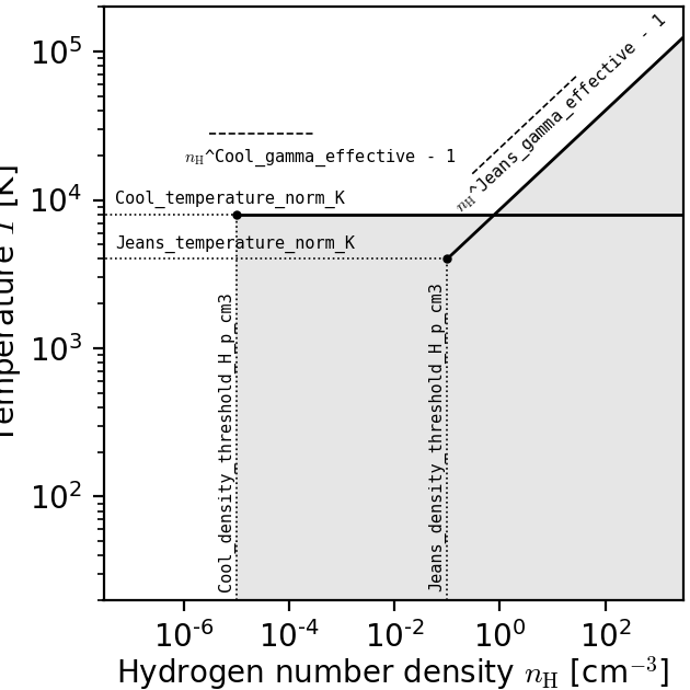
Temperature-density plane with the two entropy floors used in the EAGLE model indicated by the black lines. Gas particles are not allowed to be below either of these two floors; they are hence forbidden to enter the grey-shaded region. The floors are specified by the position in the plane of the starting point of each line (black circle) and their slope (dashed lines). The parameter names governing the behaviour of the floors are indicated on the figure. Note that unlike what is shown on the figure for clarity reasons, typical values for EAGLE runs place both anchors at the same temperature.
An additional over-density criterion above the mean baryonic density is applied to prevent gas not collapsed into structures from being affected. To be precise, this criterion demands that the floor is applied only if \(\rho_{\rm com} > \Delta_{\rm floor}\bar{\rho_b} = \Delta_{\rm floor} \Omega_b \rho_{\rm crit,0}\), with \(\Delta_{\rm floor}\) specified by the user, \(\rho_{\rm crit,0} = 3H_0/8\pi G\) the critical density at redshift zero 1, and \(\rho_{\rm com}\) the gas co-moving density. Typical values for \(\Delta_{\rm floor}\) are of order 10.
The model is governed by 4 parameters for each of the two limits. These are
given in the EAGLEEntropyFloor section of the YAML file. The parameters
are the Hydrogen number density (in \(cm^{-3}\)) and temperature (in
\(K\)) of the anchor point of each floor as well as the power-law slope
of each floor and the minimal over-density required to apply the
limit. Note that, even though the anchor points are given in terms of
temperatures, the slopes are expressed using a power-law in terms of
entropy and not in terms of temperature. For a slope of \(\gamma\) in
the parameter file, the temperature as a function of density will be
limited to be above a power-law with slope \(\gamma - 1\) (as shown on
the figure above). To simplify things, all constants are converted
to the internal system of units upon reading the parameter file.
For a normal EAGLE run, that section of the parameter file reads:
EAGLEEntropyFloor:
   Jeans_density_threshold_H_p_cm3: 0.1       # Physical density above which the EAGLE Jeans limiter entropy floor kicks in, expressed in Hydrogen atoms per cm^3.
   Jeans_over_density_threshold:    10.       # Overdensity above which the EAGLE Jeans limiter entropy floor can kick in.
   Jeans_temperature_norm_K:        8000      # Temperature of the EAGLE Jeans limiter entropy floor at the density threshold, expressed in Kelvin.
   Jeans_gamma_effective:           1.3333333 # Slope of the EAGLE Jeans limiter entropy floor
   Cool_density_threshold_H_p_cm3:  1e-5      # Physical density above which the EAGLE Cool limiter entropy floor kicks in, expressed in Hydrogen atoms per cm^3.
   Cool_over_density_threshold:     10.       # Overdensity above which the EAGLE Cool limiter entropy floor can kick in.
   Cool_temperature_norm_K:         8000      # Temperature of the EAGLE Cool limiter entropy floor at the density threshold, expressed in Kelvin.
   Cool_gamma_effective:            1.        # Slope of the EAGLE Cool limiter entropy floor
SWIFT will convert the temperature normalisations and Hydrogen number density thresholds into internal energies and densities respectively assuming a neutral gas with primordial abundance pattern. This implies that the floor may not be exactly at the position given in the YAML file if the gas has different properties. This is especially the case for the temperature limit which will often be lower than the imposed floor by a factor \(\frac{\mu_{\rm neutral}}{\mu_{ionised}} \approx \frac{1.22}{0.59} \approx 2\) due to the different ionisation states of the gas.
Recall that we additionally impose an absolute minimum temperature at all densities with a value provided in the SPH section of the parameter file. This minimal temperature is typically set to 100 Kelvin.
Note that the model only makes sense if the Cool threshold is at a lower
density than the Jeans threshold.
Chemical tracers
The gas particles in the EAGLE model carry metal abundance information in the form of metal mass fractions. We follow explicitly 9 of the 11 elements that Wiersma et al. (2009)b traced in their chemical enrichment model. These are: H, He, C, N, O, Ne, Mg, Si and Fe 2. We additionally follow the total metal mass fraction (i.e. absolute metallicity) Z. This is typically larger than the sum of the 7 metals that are individually traced since this will also contain the contribution of all the elements that are not individually followed. We note that all of definitions are independent of any definition of solar the solar metallicity \(Z_\odot\) or of any solar abundance pattern.
As part of the diagnostics, we additionally trace the elements coming from the different stellar evolution channels. We store for each particle the total mass coming from all the SNIa that enriched that particle and the metal mass fraction from SNIa. This is the fraction of the total gas mass that is in the form of metals originating from SNIa stars. By construction this fraction will be smaller than the total metal mass fraction. The same tracers exist for the SNII and AGB channels. Finally, we also compute the iron gas fraction from SNIa. This it the fraction of the total gas mass that is made of iron originating from SNIa explosions.
We finally also compute the smoothed versions of the individual element mass fractions, of the total metal mass fractions, and of the iron gas fraction from SNIa.
The chemistry module in src/chemistry/EAGLE/ includes all the arrays
that are added to the particles and the functions used to compute the
smoothed elements.
When a star is formed (see the section Star formation: Schaye+2008 modified for EAGLE below), it inherits all the chemical tracers of its parent gas particle.
In the snapshots, we output for each gas and star particle:
Name |
Description |
Units |
Comments |
|---|---|---|---|
|
Fraction of the gas/star mass
in the different elements
|
[-] |
Array of length
9 for each particle
|
|
Fraction of the gas/star mass
in the different elements
smoothed over SPH neighbours
|
[-] |
Array of length
9 for each particle
|
|
Fraction of the gas/star mass
in all metals
|
[-] |
|
|
Fraction of the gas/star mass
in all metals
smoothed over SPH neighbours
|
[-] |
|
|
Total mass of the gas/star
that was produced by enrichment
from SNIa stars
|
[U_M] |
|
|
Fraction of the total gas/star
mass that is in metals produced
by enrichment from SNIa stars
|
[-] |
|
|
Total mass of the gas/star
that was produced by enrichment
from AGB stars
|
[U_M] |
|
|
Fraction of the total gas/star
mass that is in metals produced
by enrichment from AGB star
|
[-] |
|
|
Total mass of the gas/star
that was produced by enrichment
from SNII stars
|
[U_M] |
|
|
Fraction of the gas/star mass
that is in metals produced by
enrichment from SNII stars
|
[-] |
|
|
Fraction of the total gas/star
mass in iron produced produced
by enrichment from SNIa stars
|
[-] |
|
|
Fraction of the total gas/star
mass in iron produced produced
by enrichment from SNIa stars
smoothed over SPH neighbours
|
[-] |
The stars will lose mass over their lifetime (up to ~45%). The fractions will
remain unchanged but if one is interested in computing an absolute metal mass
(say) for a star, the InitialMasses (see the section
Star formation: Schaye+2008 modified for EAGLE below) of the star must be used.
The chemistry model only requires a small number of parameters to be specified in the EAGLEChemistry section of the YAML file. These are the initial values of the metallicity and element mass fractions. These are then applied at the start of a simulation to all the gas and star particles. All 9 traced elements have to be specified An example section, for primordial abundances (typical for a cosmological run), is:
EAGLEChemistry:
  init_abundance_metal:        0.    # Mass fraction in *all* metals
  init_abundance_Hydrogen:     0.755 # Mass fraction in Hydrogen
  init_abundance_Helium:       0.245 # Mass fraction in Helium
  init_abundance_Carbon:       0.    # Mass fraction in Carbon
  init_abundance_Nitrogen:     0.    # Mass fraction in Nitrogen
  init_abundance_Oxygen:       0.    # Mass fraction in Oxygen
  init_abundance_Neon:         0.    # Mass fraction in Neon
  init_abundance_Magnesium:    0.    # Mass fraction in Magnesium
  init_abundance_Silicon:      0.    # Mass fraction in Silicon
  init_abundance_Iron:         0.    # Mass fraction in Iron
Whilst one would use the following values for solar abundances (typical for an idealised low-redshift run):
EAGLEChemistry:
  init_abundance_metal:        0.014        # Mass fraction in *all* metals
  init_abundance_Hydrogen:     0.70649785   # Mass fraction in Hydrogen
  init_abundance_Helium:       0.28055534   # Mass fraction in Helium
  init_abundance_Carbon:       2.0665436e-3 # Mass fraction in Carbon
  init_abundance_Nitrogen:     8.3562563e-4 # Mass fraction in Nitrogen
  init_abundance_Oxygen:       5.4926244e-3 # Mass fraction in Oxygen
  init_abundance_Neon:         1.4144605e-3 # Mass fraction in Neon
  init_abundance_Magnesium:    5.907064e-4  # Mass fraction in Magnesium
  init_abundance_Silicon:      6.825874e-4  # Mass fraction in Silicon
  init_abundance_Iron:         1.1032152e-3 # Mass fraction in Iron
Note that the code will verify that the input values make broad sense. This means that SWIFT checks on startup that:
\(Z_{\rm H}+Z_{\rm He}+Z_{\rm metals} \approx 1\)
\(Z_{\rm C} + Z_{\rm N} + Z_{\rm O} + Z_{\rm Ne} + Z_{\rm Mg} + Z_{\rm Si} + Z_{\rm Fe} \lesssim Z_{\rm metals}\)
\(Z_{\rm H} + Z_{\rm He} + Z_{\rm C} + Z_{\rm N} + Z_{\rm O} + Z_{\rm Ne} + Z_{\rm Mg} + Z_{\rm Si} + Z_{\rm Fe} \approx 1\)
Individual element abundances for each particle can also be read
directly from the ICs. By default these are overwritten in the code by
the values read from the YAML file. However, users can set the
parameter init_abundance_metal to -1 to make SWIFT ignore the
values provided in the parameter file:
EAGLEChemistry:
  init_abundance_metal:       -1     # Read the particles' metal mass fractions from the ICs.
The ICs must then contain values for these three fields (same as what is written to the snapshots):
Name |
Description |
Units |
Comments |
|---|---|---|---|
|
Fraction of the gas/star mass
in the different elements
|
[-] |
Array of length
9 for each particle
|
|
Fraction of the gas/star mass
in all metals
|
[-] |
|
|
Fraction of the total gas/star
mass in iron produced produced
by enrichment from SNIa stars
|
[-] |
If these fields are absent, then a value of 0 will be used for all
of them, likely leading to issues in the way the code will run.
Gas cooling: Wiersma+2009a
The gas cooling is based on the redshift-dependent tables of Wiersma et
al. (2009)a that include
element-by-element cooling rates for the 11 elements (H, He, C, N, O,
Ne, Mg, Si, S, Ca and Fe) that dominate the total rates. The tables
assume that the gas is in ionization equilibrium with the cosmic microwave
background (CMB) as well as with the evolving X-ray and UV background from
galaxies and quasars described by the model of Haardt & Madau (2001). Note that this model
ignores local sources of ionization, self-shielding and non-equilibrium
cooling/heating. The tables can be obtained from this link
which is a re-packaged version of the original tables. The code reading and interpolating the
table is located in the directory src/cooling/EAGLE/.
The Wiersma tables containing the cooling rates as a function of redshift, Hydrogen number density, Helium fraction (\(X_{He} / (X_{He} + X_{H})\)) and element abundance relative to the solar abundance pattern assumed by the tables (see equation 4 in the original paper). As the particles do not carry the mass fraction of S and Ca, we compute the contribution to the cooling rate of these elements from the abundance of Si. More specifically, we assume that their abundance by mass relative to the table’s solar abundance pattern is the same as the relative abundance of Si (i.e. \([Ca/Si] = 0\) and \([S/Si] = 0\)). Users can optionally modify the ratios used for S and Ca. Note that we use the smoothed abundances of elements for all calculations.
Above the redshift of Hydrogen re-ionization we use the extra table containing net cooling rates for gas exposed to the CMB and a UV + X-ray background at redshift nine truncated above 1 Rydberg. At the redshift or re-ionization, we additionally inject a fixed user-defined amount of energy per unit mass to all the gas particles.
In addition to the tables we inject extra energy from Helium II re-ionization using a Gaussian model with a user-defined redshift for the centre, width and total amount of energy injected per unit mass. Additional energy is also injected instantaneously for Hydrogen re-ionisation to all particles (active and inactive) to make sure the whole Universe reaches the expected temperature quickly (i.e not just via the interaction with the now much stronger UV background).
For non-cosmological run, we use the \(z = 0\) table and the interpolation along the redshift dimension then becomes a trivial operation.
The cooling itself is performed using an implicit scheme (see the theory documents) which for small values of the cooling rates is solved explicitly. For larger values we use a bisection scheme. The cooling rate is added to the calculated change in energy over time from the other dynamical equations. This is different from other commonly used codes in the literature where the cooling is done instantaneously.
We note that the EAGLE cooling model does not impose any restriction on the particles’ individual time-steps. The cooling takes place over the time span given by the other conditions (e.g the Courant condition).
Finally, the cooling module also provides a function to compute the temperature of a given gas particle based on its density, internal energy, abundances and the current redshift. This temperature is the one used to compute the cooling rate from the tables and similarly to the cooling rates, they assume that the gas is in collisional equilibrium with the background radiation. The temperatures are, in particular, computed every time a snapshot is written and they are listed for every gas particle:
Name |
Description |
Units |
Comments |
|---|---|---|---|
|
Temperature of the gas as
computed from the tables.
|
[U_T] |
The calculation is performed
using quantities at the last
time-step the particle was active
|
Note that if one is running without cooling switched on at runtime, the
temperatures can be computed by passing the --temperature runtime flag (see
Command line options). Note that the tables then have to be available as in
the case with cooling switched on.
The cooling model is driven by a small number of parameter files in the EAGLECooling section of the YAML file. These are the re-ionization parameters, the path to the tables and optionally the modified abundances of Ca and S. A valid section of the YAML file looks like:
EAGLECooling:
  dir_name:     /path/to/the/Wiersma/tables/directory # Absolute or relative path
  H_reion_z:            11.5      # Redshift of Hydrogen re-ionization
  H_reion_ev_p_H:        2.0      # Energy injected in eV per Hydrogen atom for Hydrogen re-ionization.
  He_reion_z_centre:     3.5      # Centre of the Gaussian used for Helium re-ionization
  He_reion_z_sigma:      0.5      # Width of the Gaussian used for Helium re-ionization
  He_reion_ev_p_H:       2.0      # Energy injected in eV per Hydrogen atom for Helium II re-ionization.
And the optional parameters are:
EAGLECooling:
  Ca_over_Si_in_solar:       1.0 # (Optional) Value of the Calcium mass abundance ratio to solar in units of the Silicon ratio to solar. Default value: 1.
  S_over_Si_in_solar:        1.0 # (Optional) Value of the Sulphur mass abundance ratio to solar in units of the Silicon ratio to solar. Default value: 1.
Particle tracers
Over the course of the simulation, the gas particles record some information
about their evolution. These are updated for a given particle every time it is
active. The EAGLE tracers module is located in the directory
src/tracers/EAGLE/.
In the EAGLE model, we trace the maximal temperature a particle has reached and the time at which this happened. When a star is formed (see the section Star formation: Schaye+2008 modified for EAGLE below), it inherits all the tracer values of its parent gas particle. There are no parameters to the model but two values are added to the snapshots for each gas and star particle:
Name |
Description |
Units |
Comments |
|---|---|---|---|
MaximalTemperatures |
Maximal temperature reached by
this particle.
|
[U_T]
|
|
MaximalTemperaturesScaleFactorsOR
MaximalTemperaturesTimes |
Scale-factor (cosmological runs)
or time (non-cosmological runs) at
which the maximum value was reached.
|
[-]
OR
[U_t]
|
Star formation: Schaye+2008 modified for EAGLE
The star formation is based on the pressure implementation of Schaye & Dalla Vecchia (2008) with a metal-dependent star-formation density threshold following the relation derived by Schaye (2004). Above a density threshold \(n^*_{\rm H}\), expressed in number of Hydrogen atoms per (physical) cubic centimeters, the star formation rate is expressed as a pressure-law \(\dot{m}_* = m_g \times A \times \left( 1 {\rm M_\odot}~{\rm pc^2} \right)^{-n} \times \left(\frac{\gamma}{G_{\rm N}}f_gP\right)^{(n-1)/2}\), where \(n\) is the exponent of the Kennicutt-Schmidt relation (typically \(n=1.4\)) and \(A\) is the normalisation of the law (typically \(A=1.515\times10^{-4} {\rm M_\odot}~{\rm yr^{-1}}~{\rm kpc^{-2}}\) for a Chabrier IMF). \(m_g\) is the gas particle mass, \(\gamma\) is the adiabatic index, \(f_g\) the gas fraction of the disk and \(P\) the total pressure of the gas including any subgrid turbulent terms. The star formation rate of the gas particles is stored in the particles and written to the snapshots.
Once a gas particle has computed its star formation rate, we compute the probability that this particle turns into a star using \(Prob= \min\left(\frac{\dot{m}_*\Delta t}{m_g},1\right)\). We then draw a random number and convert the gas particle into a star or not depending on our luck.
The density threshold itself has a metallicity dependence. We use the smoothed metallicity (metal mass fraction) of the gas (See Chemical tracers) and apply the relation \(n^*_{\rm H} = n_{\rm H,norm}\left(\frac{Z_{\rm smooth}}{Z_0}\right)^{n_{\rm Z}}\), alongside a maximal value. The model is designed such that star formation threshold decreases with increasing metallicity. This relationship with the YAML parameters defining it is shown on the figure below.
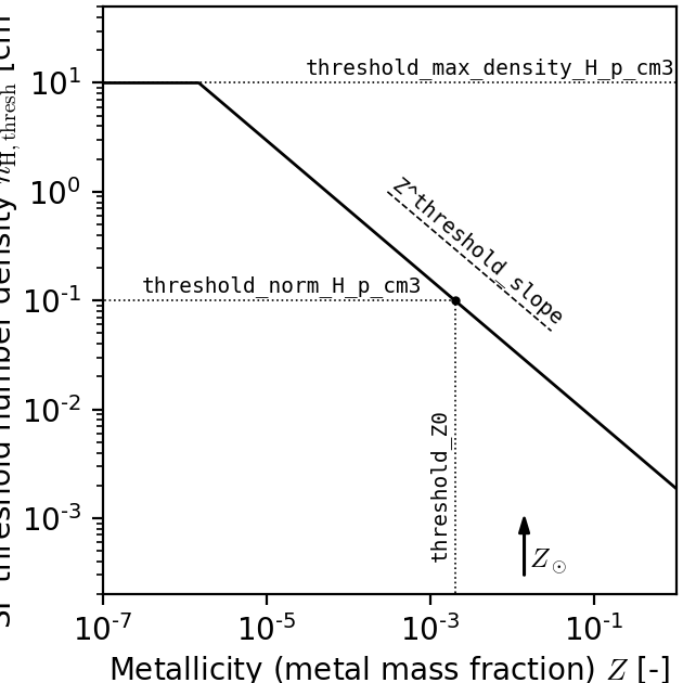
The dependency of the SF threshold density on the metallicity of the gas in the EAGLE model (black line). The function is described by the four parameters indicated on the figure. These are the slope of the dependency, its position on the metallicity-axis and normalisation (black circle) as well as the maximal threshold density allowed. For reference, the black arrow indicates the value typically assumed for solar metallicity \(Z_\odot=0.014\) (note, however, that this value does not enter the model at all). The values used to produce this figure are the ones assumed in the reference EAGLE model.
In the Schaye & Dalla Vecchia (2008) model, the pressure entering the star formation includes pressure from the unresolved turbulence. This is modeled in the form of a polytropic equation of state for the gas \(P_{EoS} = P_{\rm norm}\left(\frac{\rho}{\rho_0}\right)^{\gamma_{\rm eff}}\). For practical reasons, this relation is expressed in term of densities. Note that unlike the entropy floor, this is applied at all densities and not only above a certain threshold. This equation of state with the relevant YAML parameters defining it is shown on the figure below.
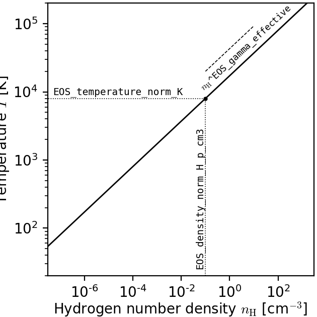
The equation-of-state assumed for the star-forming gas in the EAGLE model (black line). The function is described by the three parameters indicated on the figure. These are the slope of the relation, the position of the normalisation point on the density axis and the temperature expected at this density. Note that this is a normalisation and not a threshold. Gas at densities lower than the normalisation point will also be put on this equation of state when computing its star formation rate. The values used to produce this figure are the ones assumed in the reference EAGLE model.
In EAGLE, an entropy floor is already in use, so that the pressure of the gas is maintained high enough to prevent fragmentation of the gas. In such a scenario, there is no need for the internal EoS described above. And, of course, in such a scenario, the gas can have a pressure above the floor. The code hence uses \(P = \max(P_{\rm gas}, P_{\rm floor}, P_{\rm EoS})\).
To prevent star formation in non-collapsed objects (for instance at high redshift when the whole Universe has a density above the threshold), we apply an over-density criterion. Only gas with a density larger than a multiple of the critical density for closure can form stars.
Finally, to prevent gas much above the entropy floor (that has, for instance, been affected by feedback) from forming stars, an optional entropy margin can be specified. Only gas with an entropy \(A\) such that \(A_{\rm EoS} \leq A < A_{\rm EoS} \times 10^\Delta\), with \(\Delta\) specified in the parameter file. This defaults to a very large number, essentially removing the limit. In simulations with an entropy floor, the limit is calculated above \(\max(A_{\rm floor}, A_{EoS})\), to be consistent with the pressure used in the star formation law.
Additionally to the pressure-law corresponding to the Kennicutt-Schmidt relation described, above, we implement a second density threshold above which the slope of the relationship varies (typically steepens). This is governed by two additional parameters: the density at which the relation changes and the second slope. Finally, we optionally use a maximal density above which any gas particle automatically (i.e. direct star formation) gets a probability to form a star of 100%.
The code applying this star formation law is located in the directory
src/star_formation/EAGLE/. To simplify things, all constants are converted
to the internal system of units upon reading the parameter file.
Snapshots contain an extra field to store the star formation rates of the gas particles. If a particle was star forming in the past but isn’t any more, the field will contain negative number either corresponding to the last scale-factor where the particle was star forming (cosmological runs) or the last time where it was star forming (non-cosmological runs).
Name |
Description |
Units |
Comments |
|---|---|---|---|
|
Star formation rates of the gas if
star forming. Negative numbers
indicate the last time the gas was
star-forming.
|
[U_M / U_t] |
The quantity is not drifted so
corresponds to the rate the last
time the particle was active.
|
Note that the star formation rates are expressed in internal units and not in solar masses per year as is the case in many other codes. This choice ensures consistency between all the fields written to the snapshots.
For a normal EAGLE run, that section of the parameter file reads:
# EAGLE star formation parameters
EAGLEStarFormation:
  SF_model:                          PressureLaw
  EOS_density_norm_H_p_cm3:          0.1       # Physical density used for the normalisation of the EOS assumed for the star-forming gas in Hydrogen atoms per cm^3.
  EOS_temperature_norm_K:            8000      # Temperature om the polytropic EOS assumed for star-forming gas at the density normalisation in Kelvin.
  EOS_gamma_effective:               1.3333333 # Slope the of the polytropic EOS assumed for the star-forming gas.
  KS_normalisation:                  1.515e-4  # Normalization of the Kennicutt-Schmidt law in Msun / kpc^2 / yr.
  KS_exponent:                       1.4       # Exponent of the Kennicutt-Schmidt law.
  KS_high_density_threshold_H_p_cm3: 1e3       # Hydrogen number density above which the Kennicutt-Schmidt law changes slope in Hydrogen atoms per cm^3.
  KS_high_density_exponent:          2.0       # Slope of the Kennicutt-Schmidt law above the high-density threshold.
  gas_fraction:                      1.0       # (Optional) The gas fraction used internally by the model.
  density_direct_H_p_cm3:            1e5       # (Optional) Hydrogen number density above which a particle gets automatically turned into a star in Hydrogen atoms per cm^3. Defaults to FLT_MAX
  threshold_norm_H_p_cm3:            0.1       # Normalisation of the metal-dependant density threshold for star formation in Hydrogen atoms per cm^3.
  threshold_Z0:                      0.002     # Reference metallicity (metal mass fraction) for the metal-dependant threshold for star formation.
  threshold_slope:                   -0.64     # Slope of the metal-dependant star formation threshold
  threshold_max_density_H_p_cm3:     10.0      # Maximal density of the metal-dependant density threshold for star formation in Hydrogen atoms per cm^3.
  min_over_density:                  57.7      # Over-density above which star-formation is allowed.
  EOS_entropy_margin_dex:            0.5       # (Optional) Logarithm base 10 of the maximal entropy above the EOS at which stars can form.
Alternatively, the code can also use a simple Schmidt law for the SF rate \(\dot{m}_* = \epsilon_{ff} \times m_g \times \frac{3 \pi} {32 G \sqrt{\rho}}\), where the only free parameter is the efficiency per free-fall time \(\epsilon_{ff}\) and \(\rho\) is the density of the gas. The star-formation threshold and all the other options are applied in exactly the same way as in the pressure-law case. A valid section of the parameter file for this case reads:
# Schmidt-law star formation parameters
EAGLEStarFormation:
  SF_model:                          SchmidtLaw
  star_formation_efficiency:         0.01      # Star formation efficiency per free-fall time.
  density_direct_H_p_cm3:            1e5       # (Optional) Hydrogen number density above which a particle gets automatically turned into a star in Hydrogen atoms per cm^3. Defaults to FLT_MAX
  threshold_norm_H_p_cm3:            0.1       # Normalisation of the metal-dependant density threshold for star formation in Hydrogen atoms per cm^3.
  threshold_Z0:                      0.002     # Reference metallicity (metal mass fraction) for the metal-dependant threshold for star formation.
  threshold_slope:                   -0.64     # Slope of the metal-dependant star formation threshold
  threshold_max_density_H_p_cm3:     10.0      # Maximal density of the metal-dependant density threshold for star formation in Hydrogen atoms per cm^3.
  min_over_density:                  57.7      # Over-density above which star-formation is allowed.
  EOS_entropy_margin_dex:            0.5       # (Optional) Logarithm base 10 of the maximal entropy above the entropy floor at which stars can form.
Stellar enrichment: Wiersma+2009b
The enrichment is governed by three “master” parameters in the
EAGLEFeedback section of the parameter file. Each individual channel
can be switched on or off individually:
# EAGLE stellar enrichment master modes
EAGLEFeedback:
  use_AGB_enrichment:    1  # Global switch for enrichement from AGB stars.
  use_SNII_enrichment:   1  # Global switch for enrichement from SNII stars.
  use_SNIa_enrichment:   1  # Global switch for enrichement from SNIa stars.
Setting one of these switches to 0 will cancel the mass transfer, metal mass transfer and energy transfer (AGB only) from the stars.
The lifetime and yield tables are provided to the code via pre-computed
tables whose location is given by the filename parameter.
Choice of IMF properies
Enrichment from SNII & AGB stars
Enrichment from SNIa stars
The enrichment from SNIa is done over the lifetime of the stars and uses a
delay time distribution (DTD) to parametrize the number of SNIa events for
a star of a given age. Two functional forms are available: an exponentially
decaying function and a power-law with a slope of -1. The parameter
SNIa_DTD can hence take the two values: PowerLaw or
Exponential.
In the case of an exponential DTD, two parameters must be defined, the
normalisation (SNIa_DTD_exp_norm_p_Msun) and the time-scale
(SNIa_DTD_exp_timescale_Gyr). The original EAGLE model is reproduced by
setting the parameters to \(0.002\) and \(2.0\) respectively.
In the case of a power-law DTD, only a normalisation needs to be provided
via the parameter (SNIa_DTD_power_law_norm_p_Msun). The examples in the
repository use a value of \(0.0012\) for this.
Additionally, the age above which SNIa stars start to go off has to be
provided. Below that age, there are no explosions; above that age, the DTD
is used to determine the number of supernovae exploding in a given
time-step. This is controlled by the parameter SNIa_DTD_delay_Gyr which
sets the minimal age of SNIa in giga-years. A value of \(0.04~\rm{Gyr}
= 40~\rm{Myr}\) is used in all the examples. This corresponds
approximatively to the lifetime of stars of mass \(8~\rm{M}_\odot\).
Finally, the energy injected by a single SNIa explosion has to be provided
via the parameter SNIa_energy_erg. The canonical value of
\(10^{51}~\rm{erg}\) is used in all the examples.
The SNIa section of the YAML file for an original EAGLE run looks like:
# EAGLE-Ref SNIa enrichment and feedback options
EAGLEFeedback:
  use_SNIa_feedback:              1
  use_SNIa_enrichment:            1
  SNIa_DTD:                       Exponential
  SNIa_DTD_exp_norm_p_Msun:       0.002
  SNIa_DTD_exp_timescale_Gyr:     2.0
  SNIa_DTD_delay_Gyr:             0.04
  SNIa_energy_erg:                1.0e51
whilst for the more recent runs we use:
# EAGLE-Ref SNIa enrichment and feedback options
EAGLEFeedback:
  use_SNIa_feedback:              1
  use_SNIa_enrichment:            1
  SNIa_DTD:                       PowerLaw
  SNIa_DTD_power_law_norm_p_Msun: 0.0012
  SNIa_DTD_delay_Gyr:             0.04
  SNIa_energy_erg:                1.0e51
Supernova feedback: Dalla Vecchia+2012 & Schaye+2015
Supernova and enrichment parameters in the EAGLE-Ref model
# EAGLE stellar enrichment and feedback model
EAGLEFeedback:
  use_SNII_feedback:                1               # Global switch for SNII thermal (stochastic) feedback.
  use_SNIa_feedback:                1               # Global switch for SNIa thermal (continuous) feedback.
  use_AGB_enrichment:               1               # Global switch for enrichement from AGB stars.
  use_SNII_enrichment:              1               # Global switch for enrichement from SNII stars.
  use_SNIa_enrichment:              1               # Global switch for enrichement from SNIa stars.
  filename:                         ./yieldtables/  # Path to the directory containing the EAGLE yield tables.
  IMF_min_mass_Msun:                0.1             # Minimal stellar mass considered for the Chabrier IMF in solar masses.
  IMF_max_mass_Msun:              100.0             # Maximal stellar mass considered for the Chabrier IMF in solar masses.
  SNII_min_mass_Msun:               8.0             # Minimal mass considered for SNII stars in solar masses.
  SNII_max_mass_Msun:             100.0             # Maximal mass considered for SNII stars in solar masses.
  SNII_sampled_delay:               1               # Sample the SNII lifetimes to do feedback.
  SNII_wind_delay_Gyr:              0.03            # Time in Gyr between a star's birth and the SNII thermal feedback event when not sampling.
  SNII_delta_T_K:                   3.16228e7       # Change in temperature to apply to the gas particle in a SNII thermal feedback event in Kelvin.
  SNII_energy_erg:                  1.0e51          # Energy of one SNII explosion in ergs.
  SNII_energy_fraction_min:         0.3             # Maximal fraction of energy applied in a SNII feedback event.
  SNII_energy_fraction_max:         3.0             # Minimal fraction of energy applied in a SNII feedback event.
  SNII_energy_fraction_Z_0:         0.0012663729    # Pivot point for the metallicity dependance of the SNII energy fraction (metal mass fraction).
  SNII_energy_fraction_n_0_H_p_cm3: 1.4588          # Pivot point for the birth density dependance of the SNII energy fraction in cm^-3.
  SNII_energy_fraction_n_Z:         0.8686          # Power-law for the metallicity dependance of the SNII energy fraction.
  SNII_energy_fraction_n_n:         0.8686          # Power-law for the birth density dependance of the SNII energy fraction.
  SNIa_DTD:                         Exponential     # Functional form of the SNIa delay time distribution Two choices: 'PowerLaw' or 'Exponential'.
  SNIa_DTD_delay_Gyr:               0.04            # Stellar age after which SNIa start in Gyr (40 Myr corresponds to stars ~ 8 Msun).
  SNIa_DTD_exp_norm_p_Msun:         0.002           # Normalization of the SNIa delay time distribution in the exponential DTD case (in Msun^-1).
  SNIa_DTD_exp_timescale_Gyr:       2.0             # Time-scale of the SNIa delay time distribution in the exponential DTD case (in Gyr).
  SNIa_energy_erg:                 1.0e51           # Energy of one SNIa explosion in ergs.
  AGB_ejecta_velocity_km_p_s:      10.0             # Velocity of the AGB ejectas in km/s.
  stellar_evolution_age_cut_Gyr:    0.1             # Stellar age in Gyr above which the enrichment is down-sampled.
  stellar_evolution_sampling_rate:   10             # Number of time-steps in-between two enrichment events for a star above the age threshold.
  SNII_yield_factor_Hydrogen:       1.0             # (Optional) Correction factor to apply to the Hydrogen yield from the SNII channel.
  SNII_yield_factor_Helium:         1.0             # (Optional) Correction factor to apply to the Helium yield from the SNII channel.
  SNII_yield_factor_Carbon:         0.5             # (Optional) Correction factor to apply to the Carbon yield from the SNII channel.
  SNII_yield_factor_Nitrogen:       1.0             # (Optional) Correction factor to apply to the Nitrogen yield from the SNII channel.
  SNII_yield_factor_Oxygen:         1.0             # (Optional) Correction factor to apply to the Oxygen yield from the SNII channel.
  SNII_yield_factor_Neon:           1.0             # (Optional) Correction factor to apply to the Neon yield from the SNII channel.
  SNII_yield_factor_Magnesium:      2.0             # (Optional) Correction factor to apply to the Magnesium yield from the SNII channel.
  SNII_yield_factor_Silicon:        1.0             # (Optional) Correction factor to apply to the Silicon yield from the SNII channel.
  SNII_yield_factor_Iron:           0.5             # (Optional) Correction factor to apply to the Iron yield from the SNII channel.
Note that the value of SNII_energy_fraction_n_0_H_p_cm3 given here is
different from the value (\(0.67\)) reported in table 3 of Schaye
(2015) , as a factor
of \(h^{-2} = 0.6777^{-2} = 2.1773\) is missing in the paper.
The minimal mass for SNII stars has been raised to 8 solar masses (from 6).
Black-hole creation
Black-hole accretion
Black-hole repositioning
AGN feedback
- 1
Recall that in a non-cosmological run the critical density is set to 0, effectively removing the over-density constraint of the floors.
- 2
Wiersma et al. (2009)b originally also followed explicitly Ca and and S. They are omitted in the EAGLE model but, when needed, their abundance with respect to solar is assumed to be the same as the abundance of Si with respect to solar (See the section Gas cooling: Wiersma+2009a)